Film dosimetry#
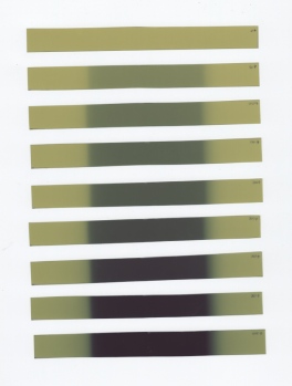
For film dosimetry, tif image must contain the irradiated film(s) and an unirradiated one, separated by a minimum distance of 5 mm between them. The color image should have three channels: red, blue and green (RGB).
This is a common example for film calibration.
Film calibration#
Start importing two libraries.
from Dosepy.image import load
from pathlib import Path
Read the tif file for film calibration and create a list with the imparted doses.
path_to_file = "/home/luis/Documentos/calibration_file.tif"
cal_image = load(path_to_file, for_calib = True)

imparted_doses = [0, 0.5, 1, 1.5, 2, 3, 5, 8, 10]
Produce the calibration curve using the red channel, a central roi with size 16 mm width, 8 mm height and a rational fit function: \(y = -c + \frac{b}{x-a}\).
cal = cal_image.get_calibration(
    doses = imparted_doses,
    channel = "R",
    roi = (16, 8),
    func = "RF"
    )
# Plot the curve
cal.plot()
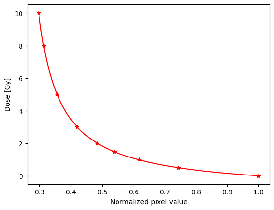
<Axes: xlabel='Normalized pixel value', ylabel='Dose [Gy]'>
Film to dose#
Load another tif file.
Note
Additionaly to the film to be transformed to dose, the scanned image must also have one unirradiated film. It is used as a reference for 0 Gy.
qa_image_path = "/home/luis/Documentos/test_file.tif"
qa_image = load(qa_image_path)
qa_image.plot()
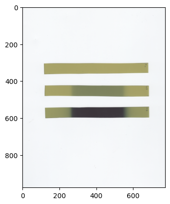
<Axes: >
Apply the calibration curve
dose_img = qa_image.to_dose(cal)
Plot it
import matplotlib.pyplot as plt
import numpy as np

fig, ax = plt.subplots(ncols=1)

max_dose = np.percentile(dose_img.array, [99.9])[0]
pos = ax.imshow(dose_img.array, cmap='nipy_spectral')
pos.set_clim(-.05, max_dose)

# add a colorbar
fig.colorbar(pos, ax=ax)
plt.plot()
[]
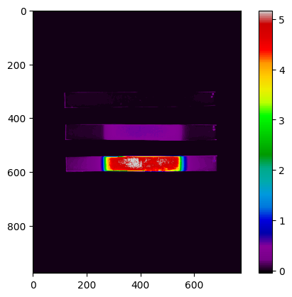
Get mean doses from central rois, 20 mm width and 8 mm hight, in each founded films.
doses_in_central_rois = qa_image.doses_in_central_rois(cal, roi = (20, 8), show=True)
print(doses_in_central_rois)
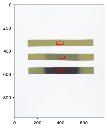
[0.009378 0.51629414 5.01072407]
Save the dose distribution as a tif file (in cGy) useful for further analysis using ImageJ.
dose_img.save_as_tif("dose_in_tif_file")
Save as csv file
# np.savetxt("some_name.txt", dose_img.array, fmt = '%.3f', delimiter = ',')