Gamma index#
For a complete description of the gamma method, see Dosepy.image.ArrayImage.gamma2D in the API section.
First we need to import Dosepy and numpy to create examples of dose distributions.
from Dosepy.image import load
import numpy as np
We generate two arrays, A and B, with the values 96 and 100 in all their elements.
a = np.zeros((30, 30)) + 96
b = np.zeros((30, 30)) + 100
To generate the dose distributions, it is only necessary to indicate the spatial resolution in dots per inch (dpi). Assuming a resolution of 25.4 dpi (1 mm), and using arrays a and b as the reference distribution and distribution to be evaluated, we execute the following commands:
D_ref = load(a, dpi = 25.4)   # Reference dose distribution
D_eval = load(b, dpi = 25.4)  # Evaluated dose distribution
Gamma comparison between two dose distributions is performed using the gamma2D method. As arguments we need:
The reference dose distribution
Dose-to-agreement [%] or [Gy].
Distance-to-agreement [mm]
On the variable D_eval, we apply the gamma2D method passing as arguments the reference distribution, D_ref, and tolerance limits (3%, 1 mm). We assign the result to the following variables:
gamma_distribution, pass_rate = D_eval.gamma2D(D_ref, 3, 1)

print(f"Pass rate: {pass_rate:.1f} %")
Pass rate: 0.0 %
By default the dose-to-agrement (3% in the example above) is relative to the maximum of the dose distribution to be evaluated. It also can be described as a local dose percentage (local normalization) calling the gamma2D method with an extra argument, local_norm.
gamma_distribution, pass_rate = D_eval.gamma2D( D_ref, 3, 1, local_norm=True)

print(f"Pass rate: {pass_rate:.1f} %")
Pass rate: 0.0 %
Since all the values in tha arrays a and b differ by 4% from each other, the pass rate is 0 for the previous two comparisons.
Dose distributions from csv files#
from Dosepy.i_o import retrieve_demo_file
film_path = "/home/luis/Documentos/D_FILM.csv"
tps_path = "/home/luis/Documentos/D_TPS.csv"
np_film = np.genfromtxt(film_path, delimiter=",", comments="#")
np_tps = np.genfromtxt(tps_path, delimiter=",", comments="#")
d_film = load(np_film, dpi=25.4)
d_tps = load(np_tps, dpi=25.4)
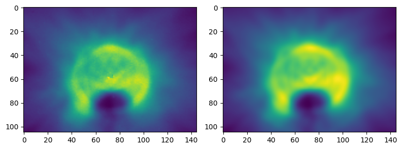
#-----------------------------------------------------
# Code to plot the dose distributions
import matplotlib.pyplot as plt
fig, axes = plt.subplots(1, 2, figsize=(8, 4))
ax = axes.ravel()
ax[0].imshow(d_film.array)
ax[1].imshow(d_tps.array)
fig.tight_layout()
plt.show()
#-----------------------------------------------------
On the d_tps distribution, we call the gamma2D method, with tolerance 3%, 2 mm, discarding all points with a dose below 10% (dose_tresh = 10). d_film will be used as the reference distribution and d_tps as the distribution to be evaluated. Limiting the distance between two points to a radius of 10 mm to reduce time computation.
g, pass_rate = d_tps.gamma2D(d_film, 3, 2, dose_threshold = 10, mask_radius = 10)

print(f'Pass rate: {pass_rate:.1f} %')
Pass rate: 98.9 %
#---------------------------------------------
#   Plotting gamma distribution

fig, axes = plt.subplots(1, 2, figsize=(12, 3))
ax = axes.ravel()

ax[0].set_title('Gamma distribution', fontsize=11)
g_im = ax[0].imshow(g, vmax=1.4)

ax[1].set_title('Gamma histogram', fontsize=11)
ax[1].grid(alpha=0.3)
ax[1].hist(g[~np.isnan(g)], bins=50, range=(0, 3), alpha=0.7, log=True)

fig.colorbar(g_im, ax=ax[0], label='Gamma')

plt.show()

Note
In order to generate easy-to-use software for users who use radiochromic film, dose distributions must meet the following characteristics:
Film dose distributions must have the same physical dimensions and spatial resolution (equal number of rows and columns) with respect to the dose distribution to be compared. You can use {py:func} ‘my_image.reduce_resolution_as(reference_image)` function to manage array size reduction.
The distributions must be registered, that is, the coordinate of a point in the reference distribution must be equal to the coordinate of the same point in the distribution to be evaluated.
Gray (Gy) and millimeters (mm) are the units used for absorbed dose and physical distance, respectively.
The dicom file must contain only a 2D dose distribution.
Dose distribution with different spatial resolution#
Create two images with different resolutions and reduce the resolution of one of them:
from Dosepy.image import load
import numpy as np

# Generate the arrays, A and B.
A = np.random.rand(100, 100)
B = np.random.rand(10, 10)

# Create the dose distributions.
D_eval = load(A, dpi = 10)
D_ref = load(B, dpi = 1)
Reduce the resolution (and array shape) of the image D_eval to have the same resolution as D_ref, using the reduce_resolution_as() method.
D_eval.reduce_resolution_as(D_ref)
Print the new shape of the D_eval array.
print(D_eval.shape) # (10, 10)

# Calculate the gamma index.
gamma_distribution, pass_rate = D_eval.gamma2D(D_ref, 3, 3)
(10, 10)